Quickstart Tutorial

multiswarm is an MPI-parallelized implementation of Particle Swarm Optimization (PSO). PSO is a method of loss minimization which starts highly explorative, and slowly reduces search space as the particles slowly decelerate and gravitate towards their personal best, and eventually the global minimum.

import jax.numpy as jnp
import numpy as np
import matplotlib.pyplot as plt

from diffopt import multiswarm

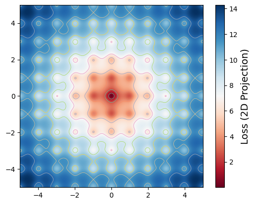
Example loss function:

The Ackley function: N-dimensional function with many local minima (roughly \(10^N\) local minima for N dimensions, each with a range of \(-5 < x_i < 5\)). Therefore, this function is essentially impossible minimize with methods like gradient descent, unless you begin with an extremely good initial guess.

def ackley(x_array):
    a = 20 * jnp.exp(-0.2 * jnp.sqrt(0.5 * (jnp.sum(x_array**2, axis=0))))
    b = jnp.exp(0.5 * jnp.sum(jnp.cos(2*jnp.pi*x_array), axis=0))
    return 20 + jnp.e - a - b


def plot_ackley2d(extent=(-5, 5, -5, 5), res=0.01,
                  ax=None, add_cbar=True):
    if ax is None:
        ax = plt.gca()
    x = np.arange(*extent[:2], res)
    y = np.arange(*extent[2:], res)
    x, y = np.meshgrid(x, y)
    z = ackley(np.array([x, y]))
    im = ax.imshow(z, cmap="RdBu", extent=extent, origin="lower")

    ax.contour(x, y, z, np.linspace(1, z.max(), 10), linewidths=0.5,
               cmap=plt.matplotlib.cm.Set2)
    if add_cbar:
        plt.colorbar(im, ax=ax).set_label("Loss (2D Projection)", fontsize=14)

plot_ackley2d()

An NVIDIA GPU may be present on this machine, but a CUDA-enabled jaxlib is not installed. Falling back to cpu.

Run PSO to minimize the loss

• Fit the 4-dimensional Ackley function

• Define search space from \(-5 < x < 5\) for all 4 dimensions

• With default inertial/cognitive/social weights, I recommend using 100 particles and iterating for 100 steps

swarm = multiswarm.ParticleSwarm(nparticles=100, ndim=4, xlow=-5, xhigh=5)
results = swarm.run_pso(ackley, nsteps=100)

PSO Progress: 100%|██████████| 100/100 [00:20<00:00,  4.96it/s]

Get the minimum loss found

• With the get_best_loss_and_params convenience function, we see that the particle swarm has converged very closely upon the global minima at the origin [0, 0, 0, 0].

best_loss, best_params = multiswarm.get_best_loss_and_params(
    results["swarm_loss_history"], results["swarm_x_history"])
print("Best loss found =", best_loss)
print("at params =", best_params)

Best loss found = -4.6277704
at params = [0.00556334 0.00865068 0.00135516 0.00539218]

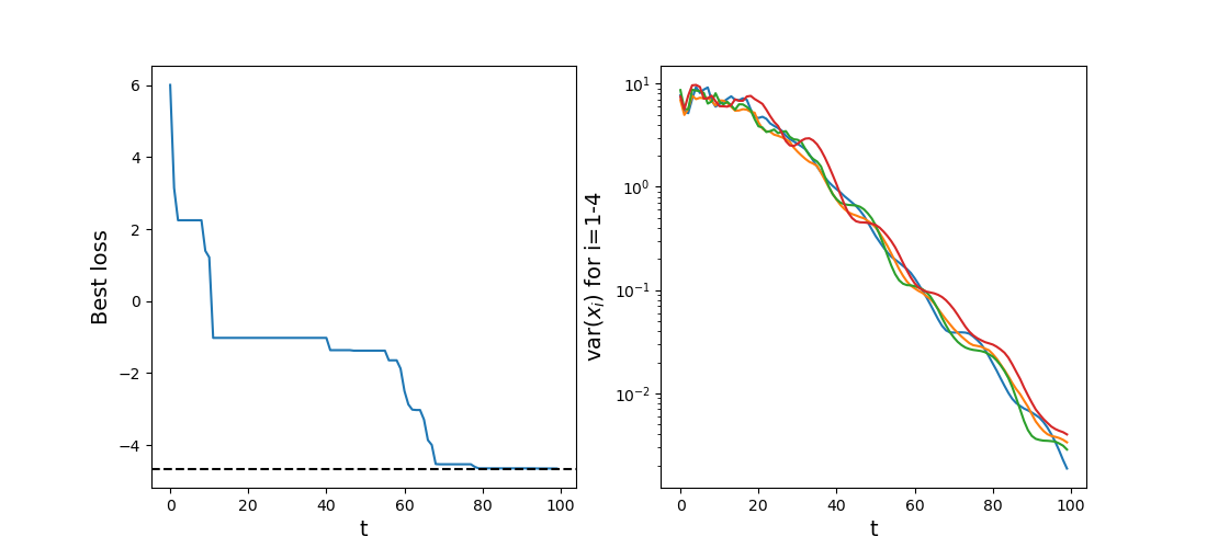
Plot the best loss as a function of time step

loss_histories = results["swarm_loss_history"]
pos_histories = results["swarm_x_history"]
best_loss_possible = ackley(np.zeros(pos_histories.shape[-1]))

var_histories = np.var(pos_histories, axis=1)
best_losses = np.min(loss_histories, axis=1)
best_losses = np.minimum.accumulate(best_losses)
fig, axes = plt.subplots(ncols=2, figsize=(11, 5))
axes[0].plot(best_losses, color="C0")
axes[0].axhline(best_loss_possible, color="k", ls="--")
axes[1].semilogy(var_histories)
axes[0].set_xlabel("t", fontsize=14)
axes[0].set_ylabel("Best loss", fontsize=14)
axes[1].set_xlabel("t", fontsize=14)
axes[1].set_ylabel("var($x_i$) for i=1-4", fontsize=14)
plt.show()

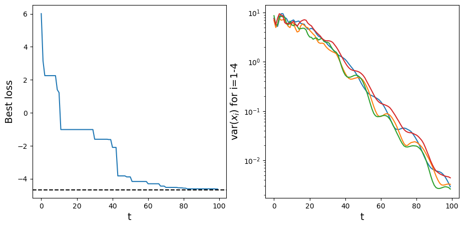
The same thing, but parallel!

multiswarm automatically distributes particles across all available MPI ranks. To try this out, let’s redo this exercise, but this time in the script multiswarm-ackley-4d.py which is copied below (this is essentially just copy-and-pasting everything we’ve done in this notebook):

"""
multiswarm-ackley-4d.py
"""

import jax.numpy as jnp
import numpy as np
import matplotlib.pyplot as plt
from mpi4py import MPI

from diffopt import multiswarm


def ackley(x_array):
    a = 20 * jnp.exp(-0.2 * jnp.sqrt(0.5 * (jnp.sum(x_array**2, axis=0))))
    b = jnp.exp(0.5 * jnp.sum(jnp.cos(2*jnp.pi*x_array), axis=0))
    return 20 + jnp.e - a - b


if __name__ == "__main__":
    swarm = multiswarm.ParticleSwarm(nparticles=100, ndim=4, xlow=-5, xhigh=5)
    results = swarm.run_pso(ackley, nsteps=100)

    best_loss, best_params = multiswarm.get_best_loss_and_params(
        results["swarm_loss_history"], results["swarm_x_history"])

    if not MPI.COMM_WORLD.rank:
        print("Best loss found =", best_loss)
        print("at params =", best_params)

        loss_histories = results["swarm_loss_history"]
        pos_histories = results["swarm_x_history"]
        best_loss_possible = ackley(np.zeros(pos_histories.shape[-1]))

        var_histories = np.var(pos_histories, axis=1)
        best_losses = np.min(loss_histories, axis=1)
        best_losses = np.minimum.accumulate(best_losses)
        fig, axes = plt.subplots(ncols=2, figsize=(11, 5))
        axes[0].plot(best_losses, color="C0")
        axes[0].axhline(best_loss_possible, color="k", ls="--")
        axes[1].semilogy(var_histories)
        axes[0].set_xlabel("t", fontsize=14)
        axes[0].set_ylabel("Best loss", fontsize=14)
        axes[1].set_xlabel("t", fontsize=14)
        axes[1].set_ylabel("var($x_i$) for i=1-4", fontsize=14)
        plt.savefig("ackley-fit-results.png")

Now let’s run this with three MPI ranks (this will assign 33-34 particles per rank). Executing mpiexec -n 3 python multiswarm-ackley-4d.py yields the following results (with about a 2x speedup on my laptop):

PSO Progress: 100%|██████████| 100/100 [00:08<00:00, 11.50it/s]
Best loss found = -4.6522627
at params = [ 0.00065104 -0.0034627  -0.00270411 -0.00358401]