Upweighting Example: The Halo Mass Function (HMF)
This notebook will loosely follow the example found in the Advanced Usage section of the tutorial. However, the stellar mass \(M_{\rm min}\) and \(M_{\rm max}\) parameters will be replaced by \(b_{\rm SHMR}\) and \(m_{\rm SMHR}\). Stellar masses will now be assigned from a fixed dataset of halo masses (such that the HMF forms a triangle distribution from \(11 < \log M_h < 14\)) and the stellar mass is assigned following the relation \(\log M_\star = b_{\rm SHMR} + m_{\rm SMHR} \log M_h\). Therefore, setting the “true” parameters of \(b_{\rm SMHR} = -2\) and \(m_{\rm SMHR} = 1\), we recover an identical distribution of stellar masses to the original model (a triangle distribution ranging from \(9 < \log M_\star < 12\)).
This example model allows us to demonstrate the implementation of “HMF upweighting”: Our generate_model() function will accept an hmf_upweights array that will represent the effective number of halos represented by each halo in logmh_table. Since our model already includes weights correspoding to quenched and star-forming predictions, we can additionally incorporate our HMF upweights by adding the following lines near the end of the function:
def generate_model(...):
    ...
    # Propagate hmf_upweights to both the Q and SF predictions
    hmf_upweights_duped = jnp.concatenate([hmf_upweights, hmf_upweights])
    # Incorporate hmf upweighting into the existing Q-vs-SF weights
    weights = weights * hmf_upweights_duped
    ...
At the end of this tutorial, we will show that we arrive at essentially identical results with and without upweighting.
[1]:
import functools
import numpy as np
import jax.numpy as jnp
import jax.random
import matplotlib.pyplot as plt
import seaborn as sns

from diffopt import kdescent
Matplotlib is building the font cache; this may take a moment.
Define the model
[2]:
model_nsample = 10_000
data_nsample = 5_000  # same volume, but undersampled below logM* < 10.5


# Generate a fixed-seed sample of halos
def load_logmh_table(undersample=False, nsample=model_nsample):
    triangle_vals = (0, 0.5, 1) if undersample else (0, 0, 1)
    logmh = jax.random.triangular(
        jax.random.key(12345), *triangle_vals, shape=(nsample,))

    logmh_min, logmh_max = 11.0, 14.0
    logmh = logmh_min + logmh * (logmh_max - logmh_min)
    return logmh


# Generate data weighted from two mass-dependent multivariate normals
@jax.jit
def generate_model(params, randkey, logmh_table, hmf_upweights=1.0):
    # Parse all 20 parameters
    # =======================
    # Intercept & slope of our linear stellar-to-halo mass relation
    b_smhr, m_smhr = params[:2]

    # Distribution parameters at lower mass bound
    mean_mmin = params[2:4]
    sigma11, sigma22 = params[4:6]
    maxcov = jnp.sqrt(sigma11 * sigma22)
    sigma12 = params[6] * maxcov
    cov_mmin = jnp.array([[sigma11, sigma12],
                          [sigma12, sigma22]])
    qfrac_mmin = params[7]
    qmean_mmin = mean_mmin + params[8:10]
    qscale_mmin = params[10]

    # Distribution parameters at upper mass bound
    mean_mmax = params[11:13]
    sigma11, sigma22 = params[13:15]
    maxcov = jnp.sqrt(sigma11 * sigma22)
    sigma12 = params[15] * maxcov
    cov_mmax = jnp.array([[sigma11, sigma12],
                          [sigma12, sigma22]])
    qfrac_mmax = params[16]
    qmean_mmax = mean_mmax + params[17:19]
    qscale_mmax = params[19]

    # Generate distribution from parameters
    # =====================================
    logm = b_smhr + m_smhr * logmh_table
    # Calculate slope of mass dependence
    logmlim = logm.min(), logm.max()
    dlogm = logmlim[1] - logmlim[0]
    dmean = (mean_mmax - mean_mmin) / dlogm
    dcov = (cov_mmax - cov_mmin) / dlogm
    dqfrac = (qfrac_mmax - qfrac_mmin) / dlogm
    dqmean = (qmean_mmax - qmean_mmin) / dlogm
    dqscale = (qscale_mmax - qscale_mmin) / dlogm
    # Apply mass dependence
    mean_sf = mean_mmin + dmean * (logm[:, None] - logmlim[0])
    cov_sf = cov_mmin + dcov * (logm[:, None, None] - logmlim[0])
    mean_q = qmean_mmin + dqmean * (logm[:, None] - logmlim[0])
    qscale = qscale_mmin + dqscale * (logm - logmlim[0])
    cov_q = cov_sf * qscale[:, None, None] ** 2
    qfrac = qfrac_mmin + dqfrac * (logm - logmlim[0])

    # Generate colors from two separate multivariate normals
    rz_sf, gr_sf = jax.random.multivariate_normal(randkey, mean_sf, cov_sf).T
    rz_q, gr_q = jax.random.multivariate_normal(randkey, mean_q, cov_q).T
    # Concatenate the quenched + star-forming values and assign weights
    data_sf = jnp.array([rz_sf, gr_sf, logm]).T
    data_q = jnp.array([rz_q, gr_q, logm]).T
    data = jnp.concatenate([data_sf, data_q])
    weights = jnp.concatenate([1 - qfrac, qfrac])

    # In case hmf_upweights is scalar, broadcast it to an array
    hmf_upweights = jnp.broadcast_to(hmf_upweights, logmh_table.shape)
    # Propagate hmf_upweights to both the Q and SF predictions
    hmf_upweights_duped = jnp.concatenate([hmf_upweights, hmf_upweights])
    # Incorporate hmf upweighting into the existing Q-vs-SF weights
    weights = weights * hmf_upweights_duped
    return data, weights

true_logmh_table = load_logmh_table()
undersampled_logmh_table = load_logmh_table(
    undersample=True, nsample=data_nsample)
Define “true” parameters to generate training data
[3]:
truth_b_smhr = -2.0
truth_m_smhr = 1.0

truth_mean_mmin = jnp.array([1.4, 1.1])
truth_var_mmin = jnp.array([0.7, 0.4])
truth_corr_mmin = 0.3
truth_qfrac_mmin = 0.2
truth_qmean_mmin = jnp.array([-0.1, 1.6])
truth_qscale_mmin = 0.3

truth_mean_mmax = jnp.array([2.0, 1.6])
truth_var_mmax = jnp.array([0.5, 0.5])
truth_corr_mmax = 0.75
truth_qfrac_mmax = 0.95
truth_qmean_mmax = jnp.array([-0.6, 1.2])
truth_qscale_mmax = 1.1

bounds_var = ([0.001, jnp.inf], [0.001, jnp.inf])
bounds_corr = [-0.999, 0.999]
bounds_qfrac = [0.0, 1.0]
bounds_qmean_gr = [0.001, jnp.inf]
bounds_qscale = [0.001, jnp.inf]

truth = jnp.array([
    truth_b_smhr, truth_m_smhr,
    *truth_mean_mmin, *truth_var_mmin, truth_corr_mmin, truth_qfrac_mmin,
    *truth_qmean_mmin, truth_qscale_mmin,
    *truth_mean_mmax, *truth_var_mmax, truth_corr_mmax, truth_qfrac_mmax,
    *truth_qmean_mmax, truth_qscale_mmax
])
guess = jnp.array([
    -3.0, 1.1, *[0.0, 0.0, 1.0, 1.0, 0.0, 0.5, 0.0, 1.0, 1.0]*2
])
bounds = [
    None, None,
    *[None, None, *bounds_var, bounds_corr, bounds_qfrac,
      None, bounds_qmean_gr, bounds_qscale]*2
]

# Generate training data from the truth parameters we just defined
truth_randkey = jax.random.key(43)
training_x_weighted, training_w = generate_model(
    truth, truth_randkey, undersampled_logmh_table)

# KDescent allows weighted training data, but to make this more realistic,
# let's generate our actual training data by randomized weighted sampling
training_selection = jax.random.uniform(
    jax.random.split(truth_randkey)[0], training_w.shape) < training_w
training_x = training_x_weighted[training_selection]
Define plotting function
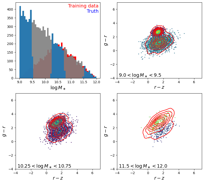
Plot the mass distribution + the color-color distribution in three separate mass bins
[4]:
lowmass_cut = [9.0, 9.5]
midmass_cut = [10.25, 10.75]
highmass_cut = [11.5, 12.0]
is_lowmass = ((lowmass_cut[0] < training_x_weighted[:, 2])
              & (training_x_weighted[:, 2] < lowmass_cut[1]))
is_midmass = ((midmass_cut[0] < training_x_weighted[:, 2])
              & (training_x_weighted[:, 2] < midmass_cut[1]))
is_highmass = ((highmass_cut[0] < training_x_weighted[:, 2])
               & (training_x_weighted[:, 2] < highmass_cut[1]))
training_w_lowmass = training_w * is_lowmass
training_w_midmass = training_w * is_midmass
training_w_highmass = training_w * is_highmass
is_noweight_lowmass = (
    (lowmass_cut[0] < training_x[:, 2])
    & (training_x[:, 2] < lowmass_cut[1]))
is_noweight_midmass = (
    (midmass_cut[0] < training_x[:, 2])
    & (training_x[:, 2] < midmass_cut[1]))
is_noweight_highmass = (
    (highmass_cut[0] < training_x[:, 2])
    & (training_x[:, 2] < highmass_cut[1]))


def generate_model_into_mass_bins(params, randkey):
    key1 = jax.random.split(randkey)[0]
    model_x, model_w = generate_model(params, key1, true_logmh_table)
    is_low = ((lowmass_cut[0] < model_x[:, 2])
              & (model_x[:, 2] < lowmass_cut[1]))
    is_mid = ((midmass_cut[0] < model_x[:, 2])
              & (model_x[:, 2] < midmass_cut[1]))
    is_high = ((highmass_cut[0] < model_x[:, 2])
               & (model_x[:, 2] < highmass_cut[1]))
    return (model_x, model_x[is_low], model_x[is_mid], model_x[is_high],
            model_w, model_w[is_low], model_w[is_mid], model_w[is_high])


def make_sumstat_plot(params, txt="", fig=None, prev_layers=None):
    (modall, modlow, modmid, modhigh,
     w_all, w_low, w_mid, w_high) = generate_model_into_mass_bins(
         params, jax.random.key(13))
    if prev_layers is not None:
        for layer in prev_layers:
            layer.remove()

    fig = plt.figure(figsize=(10, 9)) if fig is None else fig
    ax = fig.add_subplot(221) if len(fig.axes) < 4 else fig.axes[0]
    ax.hist(training_x_weighted[:, 2], bins=50, color="red",
            weights=training_w)
    _, bins, hist1 = ax.hist(
        modall[:, 2], color="grey", bins=50, alpha=0.9, weights=w_all)
    hist2 = ax.hist(modlow[:, 2], bins=list(bins), color="C0",
                    alpha=0.9, weights=w_low)[-1]
    hist3 = ax.hist(modmid[:, 2], bins=list(bins), color="C0",
                    alpha=0.9, weights=w_mid)[-1]
    hist4 = ax.hist(modhigh[:, 2], bins=list(bins), color="C0",
                    alpha=0.9, weights=w_high)[-1]
    ax.set_xlabel("$\\log M_\\ast$", fontsize=14)
    text1 = ax.text(
        0.98, 0.98, "Training data", color="red", va="top", ha="right",
        fontsize=14, transform=ax.transAxes)
    text2 = ax.text(
        0.98, 0.91, txt, color="blue", va="top", ha="right",
        fontsize=14, transform=ax.transAxes)

    ax = fig.add_subplot(222) if len(fig.axes) < 4 else fig.axes[1]
    hex1 = ax.hexbin(*modlow[:, :2].T, mincnt=1,
                     C=w_low, reduce_C_function=np.sum,
                     norm=plt.matplotlib.colors.LogNorm())
    if prev_layers is None:
        sns.kdeplot(
            {"$r - z$": training_x_weighted[is_lowmass][:, 0],
             "$g - r$": training_x_weighted[is_lowmass][:, 1]},
            weights=training_w[is_lowmass],
            x="$r - z$", y="$g - r$", color="red", levels=7, ax=ax)
    ax.set_xlabel("$r - z$", fontsize=14)
    ax.set_ylabel("$g - r$", fontsize=14)
    text3 = ax.text(
        0.02, 0.02, f"${lowmass_cut[0]} < \\log M_\\ast < {lowmass_cut[1]}$",
        fontsize=14, transform=ax.transAxes)

    ax = fig.add_subplot(223, sharex=ax, sharey=ax) if len(
        fig.axes) < 4 else fig.axes[2]
    hex2 = ax.hexbin(*modmid[:, :2].T, mincnt=1,
                     C=w_mid, reduce_C_function=np.sum,
                     norm=plt.matplotlib.colors.LogNorm())
    if prev_layers is None:
        sns.kdeplot(
            {"$r - z$": training_x_weighted[is_midmass][:, 0],
             "$g - r$": training_x_weighted[is_midmass][:, 1]},
            weights=training_w[is_midmass],
            x="$r - z$", y="$g - r$", color="red", levels=7, ax=ax)
    ax.set_xlabel("$r - z$", fontsize=14)
    ax.set_ylabel("$g - r$", fontsize=14)
    text4 = ax.text(
        0.02, 0.02, f"${midmass_cut[0]} < \\log M_\\ast < {midmass_cut[1]}$",
        fontsize=14, transform=ax.transAxes)

    ax = fig.add_subplot(224, sharex=ax, sharey=ax) if len(
        fig.axes) < 4 else fig.axes[3]
    hex3 = ax.hexbin(*modhigh[:, :2].T, mincnt=1,
                     C=w_high, reduce_C_function=np.sum,
                     norm=plt.matplotlib.colors.LogNorm())
    if prev_layers is None:
        sns.kdeplot(
            {"$r - z$": training_x_weighted[is_highmass][:, 0],
             "$g - r$": training_x_weighted[is_highmass][:, 1]},
            weights=training_w[is_highmass],
            x="$r - z$", y="$g - r$", color="red", levels=7, ax=ax)
    ax.set_xlabel("$r - z$", fontsize=14)
    ax.set_ylabel("$g - r$", fontsize=14)
    text5 = ax.text(
        0.02, 0.02, f"${highmass_cut[0]} < \\log M_\\ast < {highmass_cut[1]}$",
        fontsize=14, transform=ax.transAxes)
    ax.set_xlim(-4, 7)
    ax.set_ylim(-4, 7)
    return [hex1, hex2, hex3, hist1, hist2, hist3, hist4,
            text1, text2, text3, text4, text5]
[5]:
make_sumstat_plot(truth, txt="Truth")
plt.show()
Define loss function comparing \({\rm PDF}(g-r, r-z | M_\ast)\) and its Fourier pair
[6]:
ktrain_lowmass = kdescent.KPretrainer.from_training_data(
    training_x[is_noweight_lowmass, :2],
    bandwidth_factor=0.3, fourier_range_factor=3.0,
)
ktrain_midmass = kdescent.KPretrainer.from_training_data(
    training_x[is_noweight_midmass, :2],
    bandwidth_factor=0.3, fourier_range_factor=3.0,
)
ktrain_highmass = kdescent.KPretrainer.from_training_data(
    training_x[is_noweight_highmass, :2],
    bandwidth_factor=0.3, fourier_range_factor=3.0,
)
kcalc_lowmass = kdescent.KCalc(ktrain_lowmass)
kcalc_midmass = kdescent.KCalc(ktrain_midmass)
kcalc_highmass = kdescent.KCalc(ktrain_highmass)


# Differentiable alternative hard binning in the loss function:
@jax.jit
def soft_tophat(x, low, high, squish=25.0):
    """Approximately return 1 when `low < x < high`, else return 0"""
    width = (high - low) / squish
    left = jax.nn.sigmoid((x - low) / width)
    right = jax.nn.sigmoid((high - x) / width)
    return left * right


@jax.jit
def lossfunc(params, randkey, logmh_table=None, hmf_upweights=1.0):
    if logmh_table is None:
        logmh_table = true_logmh_table
    key1, *keys = jax.random.split(randkey, 7)
    model_x, model_w = generate_model(params, key1, logmh_table, hmf_upweights)
    weight_low = soft_tophat(model_x[:, 2], *lowmass_cut) * model_w
    weight_mid = soft_tophat(model_x[:, 2], *midmass_cut) * model_w
    weight_high = soft_tophat(model_x[:, 2], *highmass_cut) * model_w

    model_low_counts, truth_low_counts = kcalc_lowmass.compare_kde_counts(
        keys[0], model_x[:, :2], weight_low)
    model_mid_counts, truth_mid_counts = kcalc_midmass.compare_kde_counts(
        keys[1], model_x[:, :2], weight_mid)
    model_high_counts, truth_high_counts = kcalc_highmass.compare_kde_counts(
        keys[2], model_x[:, :2], weight_high)

    model_low_fcounts, truth_low_fcounts = kcalc_lowmass.compare_fourier_counts(
        keys[3], model_x[:, :2], weight_low)
    model_mid_fcounts, truth_mid_fcounts = kcalc_midmass.compare_fourier_counts(
        keys[4], model_x[:, :2], weight_mid)
    model_high_fcounts, truth_high_fcounts = kcalc_highmass.compare_fourier_counts(
        keys[5], model_x[:, :2], weight_high)

    # Convert counts to conditional prob: P(krnl | M*) = N(krnl & M*) / N(M*)
    model_low_condprob = model_low_counts / (weight_low.sum() + 1e-10)
    model_mid_condprob = model_mid_counts / (weight_mid.sum() + 1e-10)
    model_high_condprob = model_high_counts / (weight_high.sum() + 1e-10)
    truth_low_condprob = truth_low_counts / (training_w_lowmass.sum() + 1e-10)
    truth_mid_condprob = truth_mid_counts / (training_w_midmass.sum() + 1e-10)
    truth_high_condprob = truth_high_counts / (
        training_w_highmass.sum() + 1e-10)
    # Convert Fourier counts to "conditional" ECF analogously
    model_low_ecf = model_low_fcounts / (weight_low.sum() + 1e-10)
    model_mid_ecf = model_mid_fcounts / (weight_mid.sum() + 1e-10)
    model_high_ecf = model_high_fcounts / (weight_high.sum() + 1e-10)
    truth_low_ecf = truth_low_fcounts / (training_w_lowmass.sum() + 1e-10)
    truth_mid_ecf = truth_mid_fcounts / (training_w_midmass.sum() + 1e-10)
    truth_high_ecf = truth_high_fcounts / (training_w_highmass.sum() + 1e-10)

    # One constraint on number density at the highest stellar mass bin
    volume = 100.0
    model_massfunc = jnp.array([weight_high.sum(),]) / volume
    truth_massfunc = jnp.array([training_w_highmass.sum(),]) / volume

    # Must abs() the fourier-difference so the loss is real
    sqerrs = jnp.concatenate([(model_low_condprob - truth_low_condprob)**2,
                              (model_mid_condprob - truth_mid_condprob)**2,
                              (model_high_condprob - truth_high_condprob)**2,
                              jnp.abs(model_low_ecf - truth_low_ecf)**2,
                              jnp.abs(model_mid_ecf - truth_mid_ecf)**2,
                              jnp.abs(model_high_ecf - truth_high_ecf)**2,
                              (model_massfunc - truth_massfunc)**2,
                              ])

    return jnp.mean(sqerrs)
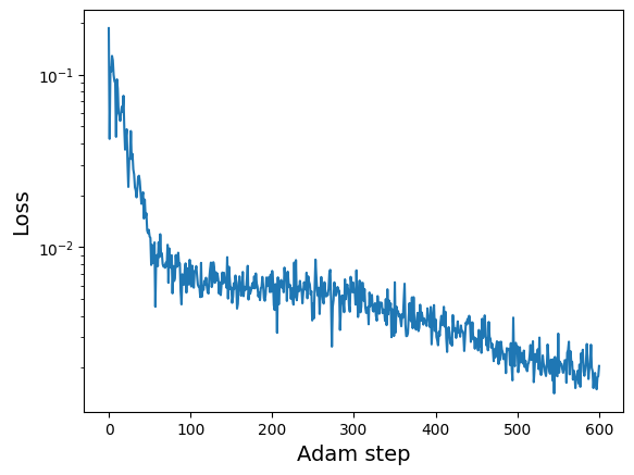
Descend the gradient without upweighting
[7]:
adam_params, adam_losses = kdescent.adam(
    lossfunc, guess, nsteps=600, param_bounds=bounds,
    learning_rate=0.03, randkey=13)
print("Best fit params =", adam_params[-1])

plt.semilogy(adam_losses)
plt.xlabel("Adam step", fontsize=14)
plt.ylabel("Loss", fontsize=14)
plt.show()
Best fit params = [-3.0341535   1.0778662   1.5392193   1.127501    0.51520944  0.35677922
  0.4562575   0.21883486 -0.17588429  1.5176885   0.38129795  1.4176784
  1.7981195   0.99692464  0.58583033  0.6330561   0.7629246   0.0794366
  1.1258303   0.8055011 ]
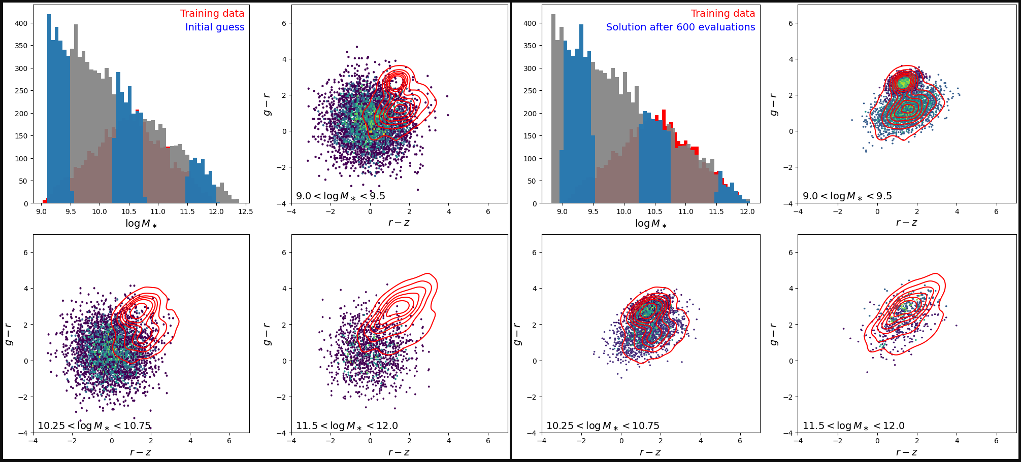
[8]:
fig = plt.figure(figsize=(20, 9), layout="constrained")
fig.set_facecolor("0.05")
figs = fig.subfigures(1, 2, wspace=0.004)
figs[0].set_facecolor("white")
figs[1].set_facecolor("white")
make_sumstat_plot(
    adam_params[0], txt="Initial guess", fig=figs[0])
make_sumstat_plot(
    adam_params[500],
    txt=f"Solution after {len(adam_params)-1} evaluations", fig=figs[1])
plt.show()

Descend the gradient with upweighting
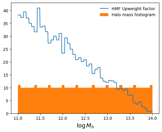
[9]:
# Define a much smaller grid of halo masses, evenly distributed so we aren't
# wasting all our computation on the many low-mass halos
evenly_spaced_logmh_table = np.linspace(11, 14, num=500)

# Define HMF upweighting using relative histogram counts - alternatively,
# you could simply use an idealized functional form for the HMF
hmf_bins = np.linspace(10.999, 14.001, num=50)
evenly_spaced_hist_counts = np.histogram(
    evenly_spaced_logmh_table, hmf_bins)[0]
true_hist_counts = np.histogram(
    true_logmh_table, hmf_bins)[0]
binned_hmf_upweights = true_hist_counts / evenly_spaced_hist_counts

# Assign HMF upweights based on the bin each "halo" falls in
bin_inds = np.digitize(evenly_spaced_logmh_table, hmf_bins) - 1
hmf_upweights = binned_hmf_upweights[bin_inds]
[10]:
# Plot HMF upweighting vs. halo mass
plt.plot(evenly_spaced_logmh_table, hmf_upweights, label="HMF Upweight factor")
plt.hist(evenly_spaced_logmh_table, bins=hmf_bins, label="Halo mass histogram")
plt.xlabel("$\\log M_h$", fontsize=14)
plt.legend(frameon=False)
plt.show()
[11]:
# Specify new halo table and HMF upweights in our new loss function
upweighted_lossfunc = functools.partial(
    lossfunc, logmh_table=evenly_spaced_logmh_table,
    hmf_upweights=hmf_upweights)

# Run gradient descent just like before (BUT ~5x FASTER!)
upweighted_adam_params, upweighted_adam_losses = kdescent.adam(
    upweighted_lossfunc, guess, nsteps=600, param_bounds=bounds,
    learning_rate=0.03, randkey=13)
print("Best fit params =", upweighted_adam_params[-1])

plt.semilogy(adam_losses)
plt.xlabel("Adam step", fontsize=14)
plt.ylabel("Loss", fontsize=14)
plt.show()
Best fit params = [-3.0093112   1.0757678   1.5629001   1.0961957   0.56475055  0.3299427
  0.43434793  0.2620157  -0.20112012  1.5347168   0.4003619   1.1400398
  1.8938192   0.90894675  0.5613661   0.49224144  0.61764735  0.36202323
  1.0692686   0.7716309 ]

[12]:
fig = plt.figure(figsize=(20, 9), layout="constrained")
fig.set_facecolor("0.05")
figs = fig.subfigures(1, 2, wspace=0.004)
figs[0].set_facecolor("white")
figs[1].set_facecolor("white")
make_sumstat_plot(
    upweighted_adam_params[0], txt="Initial guess", fig=figs[0])
make_sumstat_plot(
    upweighted_adam_params[-1],
    txt=f"Solution after {len(adam_params)-1} evaluations", fig=figs[1])
plt.show()
Closing Remarks
Neither of the fits shown here are perfect (and not even fully converged for that matter), but they are both able to qualitatively reproduce distributions that closely resemble that of the training data by eye. The power of upweighting is that we can get away with reducing compution by lowering the amount of data coming from certain regions of feature space that are over-represented, such as low halo mass bins. This allowed us to go from using 10,000 halos down to only 500 halos with HMF upweighting. This 20x reduction in data led to about a 5x reduction of compute time and memory with very similar results!