Quickstart Tutorial
kdescent provides a general framework for comparing an N-dimensional distribution of a model population to that of a training dataset. In short, it draws a mini-batched sample from the training data, computes a kernel density estimate (KDE) of the training distribution, and computes counts weighted by each mini-batched kernel (similar to computing the number density within a randomly drawn bin). These weighted counts can be directly compared to those of the model to compute a loss or
likelihood, and even perform gradient descent using Jax’s autodiff functionality. To improve the power of gradient descent even further, kdescent also provides an analogous metric for comparison of weighted counts in Fourier space. Combining both the KDE and Fourier metrics into a loss term for stochastic gradient descent has shown to be a very powerful method of parameter optimization.
[1]:
import functools
import numpy as np
import jax.numpy as jnp
import jax.random
import matplotlib.pyplot as plt

from diffopt import kdescent
Example model
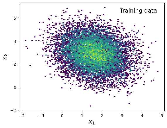
A population with variables \(x_1\) and \(x_2\) distributed as a 2D multivariate normal. We will simply parameterize this distribution with 5 parameters: [\(\mu_1\), \(\mu_2\), \(\sigma_1^2\), \(\sigma_2^2\), \(c_{12}\)] where \(\mu_i\) is the mean of each variable, \(\sigma_i^2\) is the variance of each variable, and \(c_{12}\) is the correlation coefficient between the two variables, which can be translated directly to the off-diagonal element of the covariance matrix.
[2]:
data_nsample = 10_000
model_nsample = 5_000

# Generate data from a 2D multivariate normal distribution given a
# 5-param model [mean1, mean2, sigma1**2, sigma2**2, correlation_coef]
@functools.partial(jax.jit, static_argnames=["nsample"])
def generate_data(params, randkey, nsample=model_nsample):
    mean = params[:2]
    cov11, cov22 = jnp.abs(params[2:4])
    cov12 = params[4] * jnp.sqrt(cov11 * cov22)
    cov = jnp.array([[cov11, cov12],
                     [cov12, cov22]])
    return jax.random.multivariate_normal(
        randkey, mean, cov, shape=(nsample,))
Define “true” parameters to generate training data
[3]:
truth_params = jnp.array([1.6, 2.9, 0.8, 1.25, -0.2])
truth_randkey = jax.random.key(42)

training_x = generate_data(truth_params, truth_randkey, nsample=data_nsample)

plt.hexbin(*training_x.T, mincnt=1, norm=plt.matplotlib.colors.LogNorm(),
           linewidth=0.3)
plt.text(0.95, 0.95, "Training data", fontsize=14,
         transform=plt.gca().transAxes, ha="right", va="top")
plt.xlabel("$x_1$", fontsize=14)
plt.ylabel("$x_2$", fontsize=14)
plt.show()
Define loss function comparing \({\rm PDF}(x_1, x_2)\)
Characterize the loss as the difference between our training and model distributions
We will evaluate these distributions around randomized kernel centers using the
compare_kde_countsmethod (20 kernels by default)To perform this gradient descent stochastically, the random seed for drawing kernel centers must be updated at each step. To do this, we will have our loss function accept the
randkeyargument, which it will split and pass to all sources of stochasticity
[4]:
ktrain = kdescent.KPretrainer.from_training_data(
    training_x, num_eval_kernels=20)
kde = kdescent.KCalc(ktrain)


def lossfunc(params, randkey):
    # Split random key for (1) multivariate draws and (2) kernel mini-batching
    key1, key2 = jax.random.split(randkey)
    model_x = generate_data(params, randkey=key1)
    model_kde_counts, truth_kde_counts = kde.compare_kde_counts(key2, model_x)

    # Must divide by total number in sample since the training dataset
    # is not the same size as the population generated by the model
    model_kde_density = model_kde_counts / model_nsample
    truth_kde_density = truth_kde_counts / data_nsample

    # Return the mean-squared error of our metrics
    return jnp.mean((model_kde_density - truth_kde_density)**2)
Optionally, skip the pretraining next time by writing to disk
[5]:
ktrain.save("pretrainer.npz")
ktrain = kdescent.KPretrainer.load("pretrainer.npz")
kde = kdescent.KCalc(ktrain)
Run gradient descent
[6]:
# Define initial guess and bounds for our parameters
guess = jnp.array([0., 0., 1., 1., 0.])
bounds = jnp.array([[-jnp.inf, jnp.inf], [-jnp.inf, jnp.inf],
[0.001, jnp.inf], [0.001, jnp.inf], [-0.999, 0.999]])
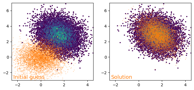
# Run gradient descent to approximately recover the truth
adam_params, adam_losses = kdescent.adam(
lossfunc, guess, nsteps=100, param_bounds=bounds,
learning_rate=1.0, randkey=12345)
print("Final params =", adam_params[-1])
print("True params =", truth_params)
Final params = [ 1.578705   2.8871017  0.7483871  1.3494768 -0.3659099]
True params = [ 1.6   2.9   0.8   1.25 -0.2 ]
[7]:
fig, axes = plt.subplots(ncols=2, figsize=(8, 3.5))

axes[0].hexbin(*training_x.T, mincnt=1, gridsize=100)
axes[0].scatter(*generate_data(guess, truth_randkey).T,
                s=1, alpha=0.3, color="C1")
axes[0].text(0.02, 0.02, "Initial guess", fontsize=13,
             color="C1", transform=axes[0].transAxes)
axes[0].set_xlim(-2.5, 4.5)
axes[0].set_ylim(-3, 7)

axes[1].hexbin(*training_x.T, mincnt=1, gridsize=100)
axes[1].scatter(*generate_data(adam_params[-1], truth_randkey).T,
                s=1, alpha=0.3, color="C1")
axes[1].text(0.02, 0.02, f"Solution", fontsize=13,
             color="C1", transform=axes[1].transAxes)
axes[1].set_xlim(-2.5, 4.5)
axes[1].set_ylim(-3, 7)
plt.show()
Advanced Usage
More complex example model
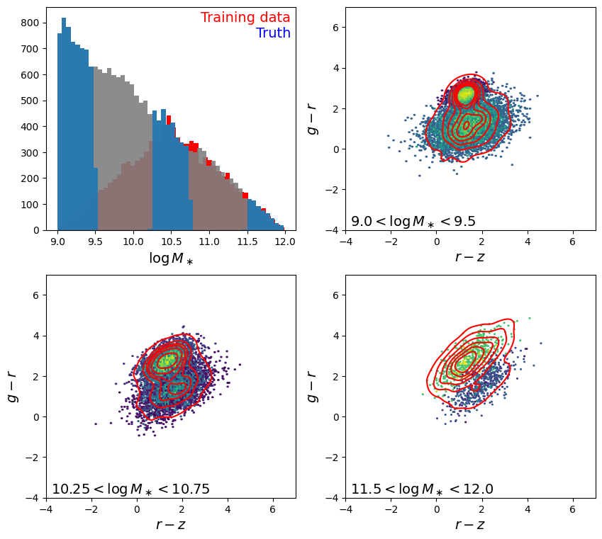
20-parameter model that generates a non-trivial bimodal 3-dimensional distribution (variables: \(\log M_\star, g-r, r-z\))
To aid our gradient descent maneuver such a tricky parameter space, we will introduce Fourier-space terms into our loss
To add even more complexity all at once: the training dataset is undersampled below \(\log M_\star < 10.5\)
We must therefore rely on conditional probability distributions \(P(g-r, r-z | \log M_\star)\), with a separate
KCalcobject handling each bin of our conditional variable, \(\log M_\star\)
[8]:
import seaborn as sns
[9]:
model_nsample = 20_000
data_nsample = 10_000  # same volume, but undersampled below logM* < 10.5

# Generate data weighted from two mass-dependent multivariate normals
@functools.partial(jax.jit, static_argnames=["undersample", "nsample"])
def generate_model(params, randkey, undersample=False, nsample=model_nsample):
    # Parse all 20 parameters
    # =======================
    # Lower and upper bounds on log stellar mass
    logmlim = params[:2]
    logmlim = logmlim.at[1].add(logmlim[0] + 0.001)

    # Distribution parameters at lower mass bound
    mean_mmin = params[2:4]
    sigma11, sigma22 = params[4:6]
    maxcov = jnp.sqrt(sigma11 * sigma22)
    sigma12 = params[6] * maxcov
    cov_mmin = jnp.array([[sigma11, sigma12],
                          [sigma12, sigma22]])
    qfrac_mmin = params[7]
    qmean_mmin = mean_mmin + params[8:10]
    qscale_mmin = params[10]

    # Distribution parameters at upper mass bound
    mean_mmax = params[11:13]
    sigma11, sigma22 = params[13:15]
    maxcov = jnp.sqrt(sigma11 * sigma22)
    sigma12 = params[15] * maxcov
    cov_mmax = jnp.array([[sigma11, sigma12],
                          [sigma12, sigma22]])
    qfrac_mmax = params[16]
    qmean_mmax = mean_mmax + params[17:19]
    qscale_mmax = params[19]

    # Generate distribution from parameters
    # =====================================
    key1, key2 = jax.random.split(randkey, num=2)
    triangle_vals = (0, 0.5, 1) if undersample else (0, 0, 1)
    logm = jax.random.triangular(key1, *triangle_vals, shape=(nsample,))
    logm = logmlim[0] + logm * (logmlim[1] - logmlim[0])
    # Calculate slope of mass dependence
    dlogm = logmlim[1] - logmlim[0]
    dmean = (mean_mmax - mean_mmin) / dlogm
    dcov = (cov_mmax - cov_mmin) / dlogm
    dqfrac = (qfrac_mmax - qfrac_mmin) / dlogm
    dqmean = (qmean_mmax - qmean_mmin) / dlogm
    dqscale = (qscale_mmax - qscale_mmin) / dlogm
    # Apply mass dependence
    mean_sf = mean_mmin + dmean * (logm[:, None] - logmlim[0])
    cov_sf = cov_mmin + dcov * (logm[:, None, None] - logmlim[0])
    mean_q = qmean_mmin + dqmean * (logm[:, None] - logmlim[0])
    qscale = qscale_mmin + dqscale * (logm - logmlim[0])
    cov_q = cov_sf * qscale[:, None, None] ** 2
    qfrac = qfrac_mmin + dqfrac * (logm - logmlim[0])

    # Generate colors from two separate multivariate normals
    rz_sf, gr_sf = jax.random.multivariate_normal(key2, mean_sf, cov_sf).T
    rz_q, gr_q = jax.random.multivariate_normal(key2, mean_q, cov_q).T
    # Concatenate the quenched + star-forming values and assign weights
    data_sf = jnp.array([rz_sf, gr_sf, logm]).T
    data_q = jnp.array([rz_q, gr_q, logm]).T
    data = jnp.concatenate([data_sf, data_q])
    weights = jnp.concatenate([1 - qfrac, qfrac])
    return data, weights
Define “true” parameters to generate training data
[10]:
truth_logmmin = 9.0
truth_logmrange = 3.0

truth_mean_mmin = jnp.array([1.4, 1.1])
truth_var_mmin = jnp.array([0.7, 0.4])
truth_corr_mmin = 0.3
truth_qfrac_mmin = 0.2
truth_qmean_mmin = jnp.array([-0.1, 1.6])
truth_qscale_mmin = 0.3

truth_mean_mmax = jnp.array([2.0, 1.6])
truth_var_mmax = jnp.array([0.5, 0.5])
truth_corr_mmax = 0.75
truth_qfrac_mmax = 0.95
truth_qmean_mmax = jnp.array([-0.6, 1.2])
truth_qscale_mmax = 1.1

bounds_truth_logmrange = [0.001, jnp.inf]
bounds_var = ([0.001, jnp.inf], [0.001, jnp.inf])
bounds_corr = [-0.999, 0.999]
bounds_qfrac = [0.0, 1.0]
bounds_qmean_gr = [0.001, jnp.inf]
bounds_qscale = [0.001, jnp.inf]

truth = jnp.array([
    truth_logmmin, truth_logmrange,
    *truth_mean_mmin, *truth_var_mmin, truth_corr_mmin, truth_qfrac_mmin,
    *truth_qmean_mmin, truth_qscale_mmin,
    *truth_mean_mmax, *truth_var_mmax, truth_corr_mmax, truth_qfrac_mmax,
    *truth_qmean_mmax, truth_qscale_mmax
])
guess = jnp.array([
    9.25, 2.5, *[0.0, 0.0, 1.0, 1.0, 0.0, 0.5, 0.0, 1.0, 1.0]*2
])
bounds = [
    None, bounds_truth_logmrange,
    *[None, None, *bounds_var, bounds_corr, bounds_qfrac,
      None, bounds_qmean_gr, bounds_qscale]*2
]

# Generate training data from the truth parameters we just defined
truth_randkey = jax.random.key(43)
training_x_weighted, training_w = generate_model(
    truth, truth_randkey, undersample=True, nsample=data_nsample)

# KDescent allows weighted training data, but to make this more realistic,
# let's generate our actual training data by randomized weighted sampling
training_selection = jax.random.uniform(
    jax.random.split(truth_randkey)[0], training_w.shape) < training_w
training_x = training_x_weighted[training_selection]
Define plotting function
Plot the mass distribution + the color-color distribution in three separate mass bins
[11]:
lowmass_cut = [9.0, 9.5]
midmass_cut = [10.25, 10.75]
highmass_cut = [11.5, 12.0]
is_lowmass = ((lowmass_cut[0] < training_x_weighted[:, 2])
              & (training_x_weighted[:, 2] < lowmass_cut[1]))
is_midmass = ((midmass_cut[0] < training_x_weighted[:, 2])
              & (training_x_weighted[:, 2] < midmass_cut[1]))
is_highmass = ((highmass_cut[0] < training_x_weighted[:, 2])
               & (training_x_weighted[:, 2] < highmass_cut[1]))
training_w_lowmass = training_w * is_lowmass
training_w_midmass = training_w * is_midmass
training_w_highmass = training_w * is_highmass
is_noweight_lowmass = (
    (lowmass_cut[0] < training_x[:, 2])
    & (training_x[:, 2] < lowmass_cut[1]))
is_noweight_midmass = (
    (midmass_cut[0] < training_x[:, 2])
    & (training_x[:, 2] < midmass_cut[1]))
is_noweight_highmass = (
    (highmass_cut[0] < training_x[:, 2])
    & (training_x[:, 2] < highmass_cut[1]))


def generate_model_into_mass_bins(params, randkey):
    key1 = jax.random.split(randkey)[0]
    model_x, model_w = generate_model(params, randkey=key1)
    is_low = ((lowmass_cut[0] < model_x[:, 2])
              & (model_x[:, 2] < lowmass_cut[1]))
    is_mid = ((midmass_cut[0] < model_x[:, 2])
              & (model_x[:, 2] < midmass_cut[1]))
    is_high = ((highmass_cut[0] < model_x[:, 2])
               & (model_x[:, 2] < highmass_cut[1]))
    return (model_x, model_x[is_low], model_x[is_mid], model_x[is_high],
            model_w, model_w[is_low], model_w[is_mid], model_w[is_high])


def make_sumstat_plot(params, txt="", fig=None, prev_layers=None):
    (modall, modlow, modmid, modhigh,
     w_all, w_low, w_mid, w_high) = generate_model_into_mass_bins(
         params, jax.random.key(13))
    if prev_layers is not None:
        for layer in prev_layers:
            layer.remove()

    fig = plt.figure(figsize=(10, 9)) if fig is None else fig
    ax = fig.add_subplot(221) if len(fig.axes) < 4 else fig.axes[0]
    ax.hist(training_x_weighted[:, 2], bins=50, color="red",
            weights=training_w)
    _, bins, hist1 = ax.hist(
        modall[:, 2], color="grey", bins=50, alpha=0.9, weights=w_all)
    hist2 = ax.hist(modlow[:, 2], bins=list(bins), color="C0",
                    alpha=0.9, weights=w_low)[-1]
    hist3 = ax.hist(modmid[:, 2], bins=list(bins), color="C0",
                    alpha=0.9, weights=w_mid)[-1]
    hist4 = ax.hist(modhigh[:, 2], bins=list(bins), color="C0",
                    alpha=0.9, weights=w_high)[-1]
    ax.set_xlabel("$\\log M_\\ast$", fontsize=14)
    text1 = ax.text(
        0.98, 0.98, "Training data", color="red", va="top", ha="right",
        fontsize=14, transform=ax.transAxes)
    text2 = ax.text(
        0.98, 0.91, txt, color="blue", va="top", ha="right",
        fontsize=14, transform=ax.transAxes)

    ax = fig.add_subplot(222) if len(fig.axes) < 4 else fig.axes[1]
    hex1 = ax.hexbin(*modlow[:, :2].T, mincnt=1,
                     C=w_low, reduce_C_function=np.sum,
                     norm=plt.matplotlib.colors.LogNorm())
    if prev_layers is None:
        sns.kdeplot(
            {"$r - z$": training_x_weighted[is_lowmass][:, 0],
             "$g - r$": training_x_weighted[is_lowmass][:, 1]},
            weights=training_w[is_lowmass],
            x="$r - z$", y="$g - r$", color="red", levels=7, ax=ax)
    ax.set_xlabel("$r - z$", fontsize=14)
    ax.set_ylabel("$g - r$", fontsize=14)
    text3 = ax.text(
        0.02, 0.02, f"${lowmass_cut[0]} < \\log M_\\ast < {lowmass_cut[1]}$",
        fontsize=14, transform=ax.transAxes)

    ax = fig.add_subplot(223, sharex=ax, sharey=ax) if len(
        fig.axes) < 4 else fig.axes[2]
    hex2 = ax.hexbin(*modmid[:, :2].T, mincnt=1,
                     C=w_mid, reduce_C_function=np.sum,
                     norm=plt.matplotlib.colors.LogNorm())
    if prev_layers is None:
        sns.kdeplot(
            {"$r - z$": training_x_weighted[is_midmass][:, 0],
             "$g - r$": training_x_weighted[is_midmass][:, 1]},
            weights=training_w[is_midmass],
            x="$r - z$", y="$g - r$", color="red", levels=7, ax=ax)
    ax.set_xlabel("$r - z$", fontsize=14)
    ax.set_ylabel("$g - r$", fontsize=14)
    text4 = ax.text(
        0.02, 0.02, f"${midmass_cut[0]} < \\log M_\\ast < {midmass_cut[1]}$",
        fontsize=14, transform=ax.transAxes)

    ax = fig.add_subplot(224, sharex=ax, sharey=ax) if len(
        fig.axes) < 4 else fig.axes[3]
    hex3 = ax.hexbin(*modhigh[:, :2].T, mincnt=1,
                     C=w_high, reduce_C_function=np.sum,
                     norm=plt.matplotlib.colors.LogNorm())
    if prev_layers is None:
        sns.kdeplot(
            {"$r - z$": training_x_weighted[is_highmass][:, 0],
             "$g - r$": training_x_weighted[is_highmass][:, 1]},
            weights=training_w[is_highmass],
            x="$r - z$", y="$g - r$", color="red", levels=7, ax=ax)
    ax.set_xlabel("$r - z$", fontsize=14)
    ax.set_ylabel("$g - r$", fontsize=14)
    text5 = ax.text(
        0.02, 0.02, f"${highmass_cut[0]} < \\log M_\\ast < {highmass_cut[1]}$",
        fontsize=14, transform=ax.transAxes)
    ax.set_xlim(-4, 7)
    ax.set_ylim(-4, 7)
    return [hex1, hex2, hex3, hist1, hist2, hist3, hist4,
            text1, text2, text3, text4, text5]
[12]:
make_sumstat_plot(truth, txt="Truth")
plt.show()
Define loss function comparing \({\rm PDF}(g-r, r-z | M_\ast)\) and its Fourier pair
[13]:
ktrain_lowmass = kdescent.KPretrainer.from_training_data(
    training_x[is_noweight_lowmass, :2],
    bandwidth_factor=0.3, fourier_range_factor=3.0,
)
ktrain_midmass = kdescent.KPretrainer.from_training_data(
    training_x[is_noweight_midmass, :2],
    bandwidth_factor=0.3, fourier_range_factor=3.0,
)
ktrain_highmass = kdescent.KPretrainer.from_training_data(
    training_x[is_noweight_highmass, :2],
    bandwidth_factor=0.3, fourier_range_factor=3.0,
)
kcalc_lowmass = kdescent.KCalc(ktrain_lowmass)
kcalc_midmass = kdescent.KCalc(ktrain_midmass)
kcalc_highmass = kdescent.KCalc(ktrain_highmass)


# Differentiable alternative hard binning in the loss function:
@jax.jit
def soft_tophat(x, low, high, squish=25.0):
    """Approximately return 1 when `low < x < high`, else return 0"""
    width = (high - low) / squish
    left = jax.nn.sigmoid((x - low) / width)
    right = jax.nn.sigmoid((high - x) / width)
    return left * right

@jax.jit
def lossfunc(params, randkey):
    key1, *keys = jax.random.split(randkey, 7)
    model_x, model_w = generate_model(params, randkey=key1)
    weight_low = soft_tophat(model_x[:, 2], *lowmass_cut) * model_w
    weight_mid = soft_tophat(model_x[:, 2], *midmass_cut) * model_w
    weight_high = soft_tophat(model_x[:, 2], *highmass_cut) * model_w

    model_low_counts, truth_low_counts = kcalc_lowmass.compare_kde_counts(
        keys[0], model_x[:, :2], weight_low)
    model_mid_counts, truth_mid_counts = kcalc_midmass.compare_kde_counts(
        keys[1], model_x[:, :2], weight_mid)
    model_high_counts, truth_high_counts = kcalc_highmass.compare_kde_counts(
        keys[2], model_x[:, :2], weight_high)

    model_low_fcounts, truth_low_fcounts = kcalc_lowmass.compare_fourier_counts(
        keys[3], model_x[:, :2], weight_low)
    model_mid_fcounts, truth_mid_fcounts = kcalc_midmass.compare_fourier_counts(
        keys[4], model_x[:, :2], weight_mid)
    model_high_fcounts, truth_high_fcounts = kcalc_highmass.compare_fourier_counts(
        keys[5], model_x[:, :2], weight_high)

    # Convert counts to conditional prob: P(krnl | M*) = N(krnl & M*) / N(M*)
    model_low_condprob = model_low_counts / (weight_low.sum() + 1e-10)
    model_mid_condprob = model_mid_counts / (weight_mid.sum() + 1e-10)
    model_high_condprob = model_high_counts / (weight_high.sum() + 1e-10)
    truth_low_condprob = truth_low_counts / (training_w_lowmass.sum() + 1e-10)
    truth_mid_condprob = truth_mid_counts / (training_w_midmass.sum() + 1e-10)
    truth_high_condprob = truth_high_counts / (
        training_w_highmass.sum() + 1e-10)
    # Convert Fourier counts to "conditional" ECF analogously
    model_low_ecf = model_low_fcounts / (weight_low.sum() + 1e-10)
    model_mid_ecf = model_mid_fcounts / (weight_mid.sum() + 1e-10)
    model_high_ecf = model_high_fcounts / (weight_high.sum() + 1e-10)
    truth_low_ecf = truth_low_fcounts / (training_w_lowmass.sum() + 1e-10)
    truth_mid_ecf = truth_mid_fcounts / (training_w_midmass.sum() + 1e-10)
    truth_high_ecf = truth_high_fcounts / (training_w_highmass.sum() + 1e-10)

    # One constraint on number density at the highest stellar mass bin
    volume = 100.0
    model_massfunc = jnp.array([weight_high.sum(),]) / volume
    truth_massfunc = jnp.array([training_w_highmass.sum(),]) / volume

    # Must abs() the Fourier residuals so that the loss is real
    sqerrs = jnp.concatenate([
        (model_low_condprob - truth_low_condprob)**2,
        (model_mid_condprob - truth_mid_condprob)**2,
        (model_high_condprob - truth_high_condprob)**2,
        jnp.abs(model_low_ecf - truth_low_ecf)**2,
        jnp.abs(model_mid_ecf - truth_mid_ecf)**2,
        jnp.abs(model_high_ecf - truth_high_ecf)**2,
        (model_massfunc - truth_massfunc)**2,
    ])

    return jnp.mean(sqerrs)
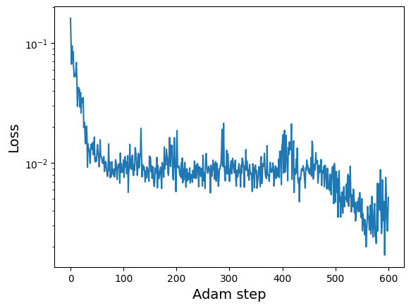
Run gradient descent
[14]:
adam_params, adam_losses = kdescent.adam(
    lossfunc, guess, nsteps=600, param_bounds=bounds,
    learning_rate=0.05, randkey=12345)
print("Best fit params =", adam_params[-1])

plt.semilogy(adam_losses)
plt.xlabel("Adam step", fontsize=14)
plt.ylabel("Loss", fontsize=14)
plt.show()
Best fit params = [ 9.2615385   2.6516986   1.4330685   1.1343558   0.36523223  0.35466456
  0.17270456  0.2798898  -0.15260133  1.5365064   0.41886896  1.2801453
  1.7342998   1.1486027   0.8496331   0.7393313   0.90481573  0.25919464
  1.1972123   0.86743474]
[15]:
fig = plt.figure(figsize=(20, 9), layout="constrained")
fig.set_facecolor("0.05")
figs = fig.subfigures(1, 2, wspace=0.004)
figs[0].set_facecolor("white")
figs[1].set_facecolor("white")
make_sumstat_plot(
    adam_params[0], txt="Initial guess", fig=figs[0])
make_sumstat_plot(
    adam_params[-1],
    txt=f"Solution after {len(adam_params)-1} evaluations", fig=figs[1])
plt.show()
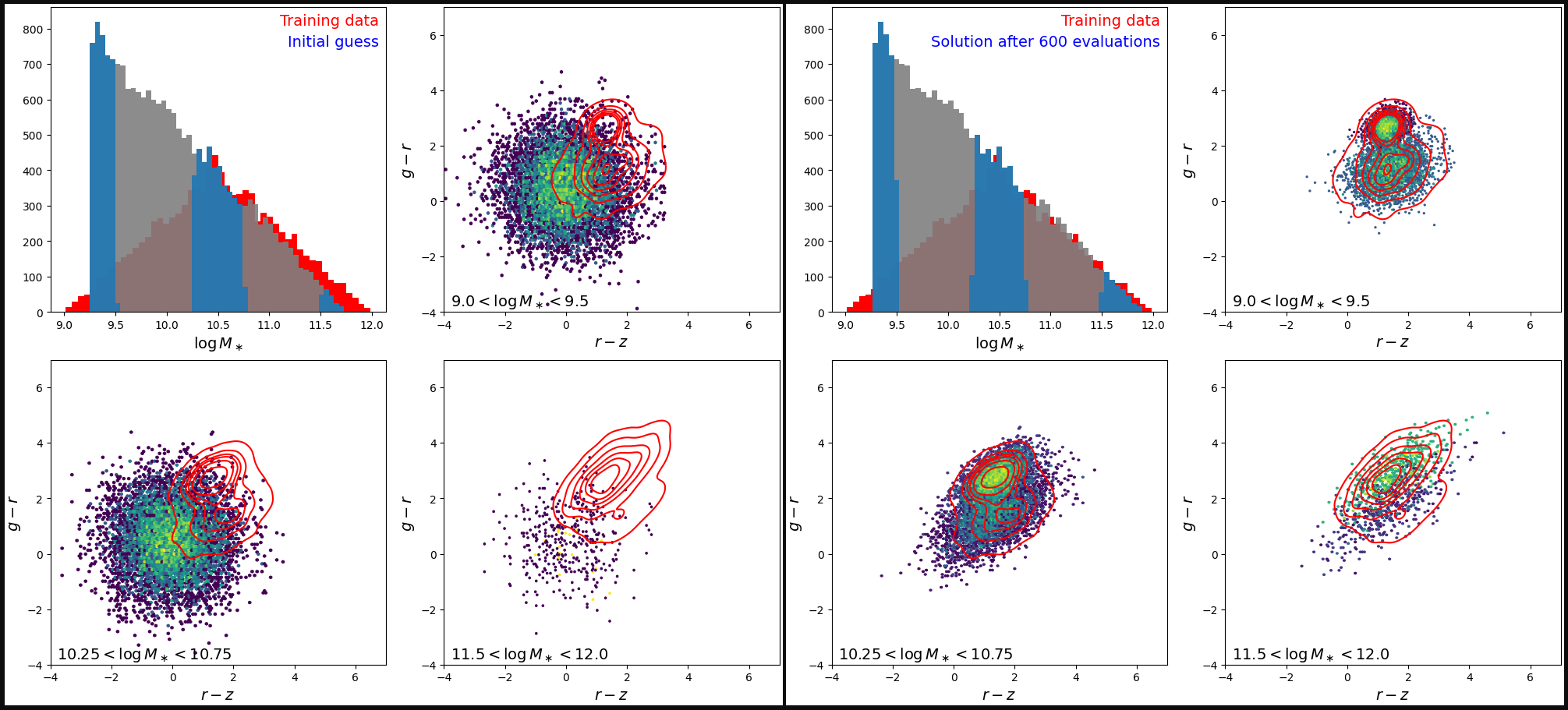
This is not a perfect fit (although it would continue to improve a little if we ran gradient descent even longer), but our goal to qualitatively recover the target distribution was a success! This shows how powerful kdescent’s Fourier counts can be as a complementary summary statistic to the PDF counts.